3가지 network 모델 종류
real-world network와 유사한 network를 생성하기 위한 network model 3개
1. Random graphs
2. Small-World Model
3. Preferential Attachment
Random graphs
가정: edge는 random하게 형성된다.
a. G(n,p)
n: node의 개수(고정)
이 때, 총 nC2만큼의 노드를 생성할 수 있는데,
이때의 edge 생성 확률을 p라고 함
따라서, 0<= edge의 개수 <= nC2
eg) p=0.2 이면 대략 edge의 개수는 nC2*0.2개임
b. G(n,m)
m: edge의 개수(고정)
모든 가능한 집합에서의 edge의 개수임 (nC2)

|Ω|만큼의 서로 다른 그래프가 존재할 수 있음
(n개의 노드와 m개의 edge로 구성된)
그 중 하나의 |Ω|그래프가 선택될 확률은 1/ |Ω| 임.
G(n,p)와 G(n,m)의 유사성
n이 커지면 커질 수록 두개의 그래프는 유사해진다.
G(n,p)와 G(n,m)의 차이점
G(n,p)에서 edge의 개수는 고정되지 않음
G(n,p)의 expected degree
: the expected number of edges connected to a node
: node와 연결된 edge의 기대값 c=(n-1)*p
→ n-1개의 edge를 p만큼의 확률로 가질 수 있으므로
→ p=c / (n-1)
G(n,p)에서 m개의 edge를 가질 확률
Evloution of Random Graph
p가 증가할수록 complete한 그래프가 되고
p가 감소할 수록 sparse한 그래프가 됨
→ p가 클수록 giant component가 될 가능성이 높다.
( Giant component= largest connected component)
Phase Transition: 어느순간부터 diameter가 줄어드는 순간이 존재함
average node degree C=1이 되는 순간
(or p=1/(n-1)인 순간, G(n,p)의 expected degree 참고)
즉 위의 회색표시 칸에서
p=1/(10-1) = 0.11일때 임
이때 diameter가 max값에 도달함
random graph의 특성
Degree Distribution
여기서, connected 그래프에서 degree가 0이 될 확률은
이 값은 1/n 보다 작아야함
이 값을 이용하여 threshold를 구할 수 있음
p가 connectivity threshold 값 이상을 가질 때는 random 그래프에서 모든 노드가 연결 되어 있음
단, threshold보다 작은 값이면 연결안된 노드들이 있다는 뜻임
G(n,p)로 생성된 random graph에서
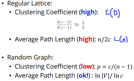
local/global clustering coefficient의 기대값=p 이다.
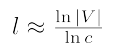
average path length 는 아래와 같다.
G(n,p)인 random graph를 만들때,
p=c/(n-1)로 정한다.
Modeling random graph
1. real world graph를 통해 평균 c(degree)값을 계산
2. c/(n-1)=p를 이용하여 p값을 계산
3. 확률 p를 이용하여 random graph를 생성
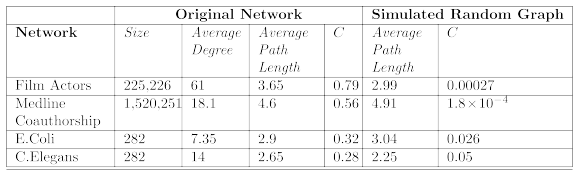
How representative is the generated graph?
[Degree Distribution] power-law degree distribution 를 따르지 않음
[Average Path Length] 는 real-world graph와 유사함
[Clustering Coefficient] real-world graph의 clustering coefficient값 보다 현저히 낮음
→ 인공적으로 random graph를 만들었을 때는
average path length만 특징이 real-world와 유사하나,
degree distribution과 cluster coefficient는 real-world와 다른 특징을 보임.
small-world model의 특징
• Short average path length
• High clustering coefficient
real-world interaction에서는 각각의 개인이 제한/고정된 number of connections을 가짐
→ regular network와 유사함
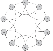
단 regular lattice를 만들기 위해서는 아래 조건을 만족해야함
(regular lattice는 특정한 패턴을 가지고 연결되어있음)
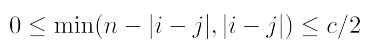
i=7, j=9이면 min(10-|7-9|, |7-9|) <= 4/2 (O)
i=7, j=1이면 min(10-|7-1|, |7-1|) <= 4/2 (X)
즉, V7과 V1은 연결하면 안됨
regular lattice network의 특징
• average path length는 높다.
• clustering coefficient는 높다.
→ 기존 small world model과 1번 가정이 다름
→ regular lattice를 수정하여 small world model과 유사하게 만들기
→ beta 값 만큼의 확률로 random하게 node를 연결하자(re-wiring)
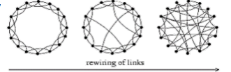
– When beta is 0, the model is basically a regular lattice
– When beta = 1, the model becomes a random graph
regular lattice network의 degree 분포
생성된 small world network의 degree분포는
모든 노드끼리 유사한 값을 가짐
→ lattice를 가지고 변형해서 만들었기 때문에
Regular lattice vs. Random Graph 비교
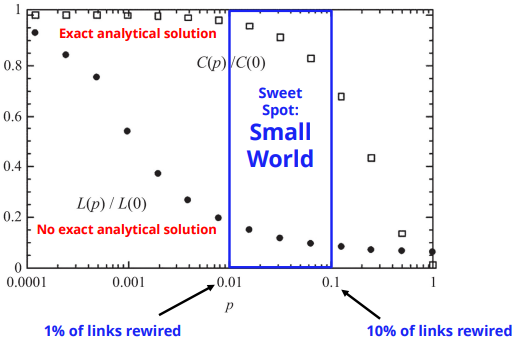
beta가 변할때, clustering coefficient와 average distance 변화량 관찰
• beta를 여기서 p라고 하고,
• L(0) is the average path length of the regular lattice
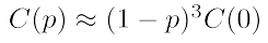
• C(0) is the clustering coefficient of the regular lattice
→ beta(P)가 조금씩 증가하면 average path length가 급격히 줄어듬
→ beta(P)가 증가하면 clustering coefficient가 초반에 완만히 줄어듬
small world graph로 생성시킨 결과
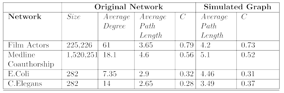
→ real world 그래프와 유사도가 높음
small world의 clustering coefficient
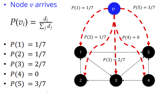
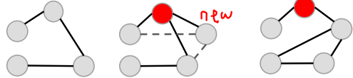
Preferential Attachment model
→ degree가 높은쪽은 degree 더 높게,
degree가 낮은쪽은 degree 더 낮게 만드는 모델임
아래그림의 예시를 참고
Preferential Attachment model로 생성한 모델의 특징(결과)
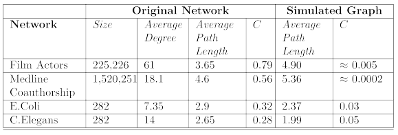
→ clustering coefficient 값이 real world 와 비교 했을 때 너무 낮음
Rich-Get-Richer Effects 설명
초기단계에서 큰 인기를 얻기는 힘들다 (preferential attachment의 단점)
(초기단계상태에서는 불안정함)
시간이 지나서 우선 rich해지면 더 빨리 rich상태에 도달 할 수 있음
preferential attachment 특징
[Degree Distribution] power-law degree distribution 를 따름
[Average Path Length] 는 real-world graph와 유사함
[Clustering Coefficient] real-world graph의 clustering coefficient값 보다 현저히 낮음
Network Models Extended
- Configuration Model
- Kleinberg Small-World Model (skip)
- Vertex Copying Model
1. Configuration Model (random graph의 확장편)
기존 random graph의 문제를 해결해보자
random graph의 문제점: the degree distribution in random graphs is not power law
해결책: (아래 그림 참고)
1. 각 노드마다 degree를 부여해줌 (stub)
- real world graph를 참고하여 부여하기
- power law 법칙을 참고하여 부여하기
2. 각 stub을 matching 시킴
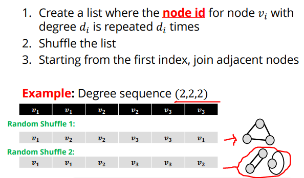
단, degree sequence의 총합은 짝수여야함 2+2+2
3. Vertex Copying Model
Basic idea:
– A new node comes in
– We select some other node at random
– We connect to that node (optional)
– We copy all of its connections
문제점:
새로들어온 노드와 연결된 노드의 edge가 없을경우 copy하는 edge가 없음
해결책: 그럴 때는 또다른 노드와 random하게 연결하자.
'IT > SNS분석' 카테고리의 다른 글
| community analysis 1 (0) | 2022.05.17 |
|---|---|
| Classification with Network Information (0) | 2022.05.10 |
| Network models1 - real world network 특징 (0) | 2022.05.02 |
| [SNS analysis]Network measures2 (0) | 2022.04.12 |
| Network measures 1 (2) | 2022.03.29 |